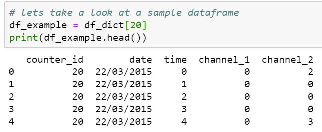
Now we have obtained our dataset from the Edinburgh Open Data store, we need to tidy it up and see if we need to transform any of the data to help us to extract meaning from it. Looking at the information on the website we are informed “Data sets have 2 or 4 channel counters (due to the width of the road), recording the direction of travel, such as north-bound, south-bound, east-bound or west-bound. Counts are on an hourly basis“. Unfortunately when we look inside the datasets no indication of direction is actually given for most of the different channels on the counters, it will likely need to be inferred from the traffic patterns on the different channels (since logically we would expect traffic to head to the city centre in the morning and away in the afternoon). Also the counters do not all have the same number of channels so we will need to be careful about how we join the dataframes.
Worse still we can see that for some locations two separate counters were used, one in each direction, but apparently only using channel one in each case. We need to tidy those dual locations into single dataframes before we can proceed
# We need to combine the data for some paired location locations [(38, 39), (40, 41), (44, 45)]
# however we need to ensure that the correct date time information is preserved
# so lets add datetime information to our dataframes and clean our dataframes up
df_dict_times = {}

for key, data in df_dict.items():
    #lets convert the date column to date-time format
    data['date_dt'] = pd.to_datetime(data['date'], format='%d/%m/%Y')
    data['timedelta'] = pd.to_timedelta(data['time'], unit = 'h')
    data['datetime'] = data['date_dt'] + data['timedelta']

# now we can take the pairs of atypical counters and combine them on the datetime column
# delete the column 2 values from both dataframes as they appear to be spurious
pairs = [(38,39),(40,41), (44,45)]

for tup in pairs:
    north = df_dict[tup[0]].drop("channel_2", axis = 1)
    south = df_dict[tup[1]].drop("channel_2", axis = 1)
    # rename south's channel_1 to channel_2 to prevent collisions
    south.rename(columns={'channel_1': 'channel_2'}, inplace=True)
    # and drop all columns except channel_2 and datetime
    south = south.drop(["time","counter_id", "timedelta","date", "date_dt"], axis = 1)
    # now merge the dataframes
    merged = pd.merge(north, south, on='datetime')
    # reinsert the merged data frame 38, 40, 44
    df_dict[tup[0]] = merged
    # and finally delete the excess dataframe 39, 41, 45
    df_dict.pop(tup[1])
Next we want to make sure that we have a common format for all the data frames so we need to amend the 2 channel dataframes to resemble the 4 channel ones. While we are doing this we can also sum the travel in each direction to get some aggregate data.
# now that we have combined this sensor data we need to do a little more tidying
for key, df_example in df_dict.items():
    # add channel_3 and channel 4 if they do not already exist
    # Note that it would appear that 4 channel roads seem to be arranged (1,2) (3,4)
    #so move channel 2 to channel 4 for consistency
    if 'channel_4' not in df_example:
        df_example['channel_3'] = 0 # add empty channel
        df_example['channel_4'] = df_example['channel_2'] # move channel 2
        df_example['channel_2'] = 0 # 0 out old values
    # add direction columns A and B totalling travel
    df_example['direction_A'] = df_example['channel_1'] + df_example['channel_2']
    df_example['direction_B'] = df_example['channel_3'] + df_example['channel_4']

# and tidy the dataframes so the columns run in the same order
df_example = df_example[['counter_id', 'date', 'time', 'datetime', 'channel_1', 'channel_2',
                         'channel_3', 'channel_4', 'direction_A', 'direction_B']]
Once this is done the dataframes are nicely compatible so we can combine them into one large dataframe for easier comparison and analysis
# finally we can combine all our separate dataframes into one giant dataframe
# to allow for some deeper analysis
# convert our dictionary of dataframes to a list
df_list = list(df_dict.values())

# then we can concatenate it
bike_df = pd.concat(df_list, ignore_index=True, sort=False)
We can also consider what other features we might like to engineer. One of the most obvious is to convert the date and hour columns into a datetime column because this will allow us to use datetime’s features to extract day and month information which is useful when analysing traffic patterns. An important point to note is that you cannot add two datetime’s together, therefore we will need to convert the hours column to timedelta format so that it can be added to the date. Another obvious column to add is a total of all traffic regardless of direction. While this can be calculated from other columns, having it in its own column allows easy use of the pivot_table command
# lets add day of the week
bike_df["Day_no"] = bike_df["datetime"].dt.dayofweek
bike_df["Day"] = bike_df["datetime"].dt.weekday_name
# add the years of the survey
bike_df["Year"] = bike_df["datetime"].dt.year

# add a month column
bike_df["Month"] = bike_df["datetime"].dt.month

# and add a total trips column
bike_df["Total"] = bike_df["direction_A"] + bike_df["direction_B"]
Hooray, our data is all cleaned, tidied and ready to be visualised. Here data cleaning has been presented as the first task, though in practise data cleaning often runs side by side with visualisation. This is because unexpected visualisation results lead us to realise issues in the data set or opportunities for feature engineering to allow us to get the most out of our data.