Previously this series has covered acquiring and preparing a dataset for image recognition using machine learning. Now that we have our data properly structured in folders for our algorithm to learn from, it is time to implement the algorithm. We are going to use the pretrained VGG16 network which was trained on the ImageNet database by the lovely people at the Visual Geometry Group. As we wish to classify different categories to the ones the network was originally trained on we are only going to use the initial layers of thei s pretrained network in a process called transfer learning. For the final layers we will train some new layers which we will add when we build the model. Overall the process can be summarised as follows
![]()
The implementation of VVG16 needs Keras and TensorFlow to run so lets start by importing the libraries we are going to need. As there is an excellent pre-existing tutorial on using VGG16 for multiclass learning we will use that code with some modifications
import numpy as np
from keras.preprocessing.image import ImageDataGenerator, img_to_array, load_img
from keras.models import Sequential
from keras.layers import Dropout, Flatten, Dense
from keras import applications
from keras.utils.np_utils import to_categorical
import matplotlib.pyplot as plt
import math
import cv2
import os
#import PIL
from PIL import Image
Next we need to set up some of the initial parameters for our algorithm
# dimensions of our images.
img_width, img_height = 224, 224

print (os.getcwd())
path = "C:/Users/Justin/Pictures/Lego"
os.chdir(path)
print (os.getcwd())

top_model_weights_path = 'bottleneck_fc_model.h5'
train_data_dir = 'data/train'
validation_data_dir = 'data/validation'

# number of epochs to train top model
epochs = 50
# batch size used by flow_from_directory and predict_generator
batch_size = 16
Once this is done it is time to start setting up the model for training, first lets import the structure and weights for the VGG16 model. Note the key line :
model = applications.VGG16(include_top=False, weights=’imagenet’)
This imports the model with the appropriate weights, but also imports it without the final layers of the model so that we can add our own. Next we specify the target directories and create generators to flow our data from the directories to the model for training and validation.
def save_bottlebeck_features():
    # build the VGG16 network
    model = applications.VGG16(include_top=False, weights='imagenet')

    datagen = ImageDataGenerator(rescale=1. / 255)

    generator = datagen.flow_from_directory(
        train_data_dir,
        target_size=(img_width, img_height),
        batch_size=batch_size,
        class_mode=None,
        shuffle=False)

    print(len(generator.filenames))
    print(generator.class_indices)
    print(len(generator.class_indices))

    nb_train_samples = len(generator.filenames)
    num_classes = len(generator.class_indices)

    predict_size_train = int(math.ceil(nb_train_samples / batch_size))

    bottleneck_features_train = model.predict_generator(
        generator, predict_size_train)

    np.save('bottleneck_features_train.npy', bottleneck_features_train)

    generator = datagen.flow_from_directory(
        validation_data_dir,
        target_size=(img_width, img_height),
        batch_size=batch_size,
        class_mode=None,
        shuffle=False)

    nb_validation_samples = len(generator.filenames)

    predict_size_validation = int(
        math.ceil(nb_validation_samples / batch_size))

    bottleneck_features_validation = model.predict_generator(
        generator, predict_size_validation)

    np.save('bottleneck_features_validation.npy',
        bottleneck_features_validation)
Running the above code saves two files ‘bottleneck_features_train.npy’ and ‘bottleneck_features_validation.npy’. As we are not planning to retrain these layers of the network, the outputs from them will be static for a given image during training, so by saving the outputs rather than recalculating them for every pass, we can speed up training.
Now we need to define the new part of the model which will be specific to our data and which will be trained to output the correct category when we feed it the data output by the trained layers of the underlying VGG16 network. We know how to structure this model, just structure it like the output layers of the original VGG16 network. This code will also include some monitoring and output functionality to let us see how our model is doing
def train_top_model():
    datagen_top = ImageDataGenerator(rescale=1. / 255)
    generator_top = datagen_top.flow_from_directory(
        train_data_dir,
        target_size=(img_width, img_height),
        batch_size=batch_size,
        class_mode='categorical',
        shuffle=False)

    nb_train_samples = len(generator_top.filenames)
    num_classes = len(generator_top.class_indices)

    # save the class indices to use use later in predictions
    np.save('class_indices.npy', generator_top.class_indices)

    # load the bottleneck features saved earlier
    train_data = np.load('bottleneck_features_train.npy')

    # get the class labels for the training data, in the original order
    train_labels = generator_top.classes

    # https://github.com/fchollet/keras/issues/3467
    # convert the training labels to categorical vectors
    train_labels = to_categorical(train_labels, num_classes=num_classes)

    generator_top = datagen_top.flow_from_directory(
        validation_data_dir,
        target_size=(img_width, img_height),
        batch_size=batch_size,
        class_mode=None,
        shuffle=False)

    nb_validation_samples = len(generator_top.filenames)

    validation_data = np.load('bottleneck_features_validation.npy')

    validation_labels = generator_top.classes
    validation_labels = to_categorical(
    validation_labels, num_classes=num_classes)

    # add the top layers to the model
    model = Sequential()
    model.add(Flatten(input_shape=train_data.shape[1:]))
    model.add(Dense(256, activation='relu'))
    model.add(Dropout(0.5))
    model.add(Dense(num_classes, activation='sigmoid'))

    model.compile(optimizer='rmsprop',
    loss='categorical_crossentropy', metrics=['accuracy'])

    history = model.fit(train_data, train_labels,
    epochs=epochs,
    batch_size=batch_size,
    validation_data=(validation_data, validation_labels))

    model.save_weights(top_model_weights_path)

    (eval_loss, eval_accuracy) = model.evaluate(
    validation_data, validation_labels, batch_size=batch_size, verbose=1)

    print("[INFO] accuracy: {:.2f}%".format(eval_accuracy * 100))
    print("[INFO] Loss: {}".format(eval_loss))

    plt.figure(1)

    # summarize history for accuracy
    plt.subplot(211)
    plt.plot(history.history['acc'])
    plt.plot(history.history['val_acc'])
    plt.title('model accuracy')
    plt.ylabel('accuracy')
    plt.xlabel('epoch')
    plt.legend(['train', 'test'], loc='upper left')

    # summarize history for loss
    plt.subplot(212)
    plt.plot(history.history['loss'])
    plt.plot(history.history['val_loss'])
    plt.title('model loss')
    plt.ylabel('loss')
    plt.xlabel('epoch')
    plt.legend(['train', 'test'], loc='upper left')
    plt.show()
Now we can train our network by running these two functions
#train the model
save_bottlebeck_features()
train_top_model()
Running the model for 10 epochs provides the following output
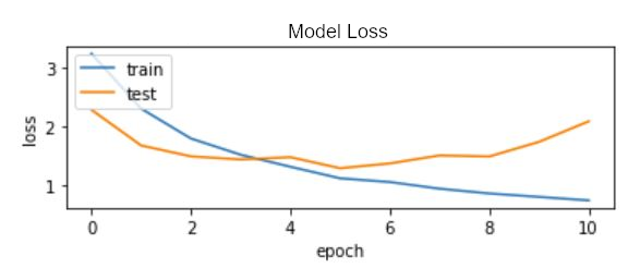
It can be seen that the test set initially provides surprisingly low loss, however around epoch 5 or 6 the loss for the validation set (here labelled as test) reaches a minimum and begins to climb again. This is a classic sign of over fitting and the simplest way to avoid it is by early stopping. Checking the logs we find
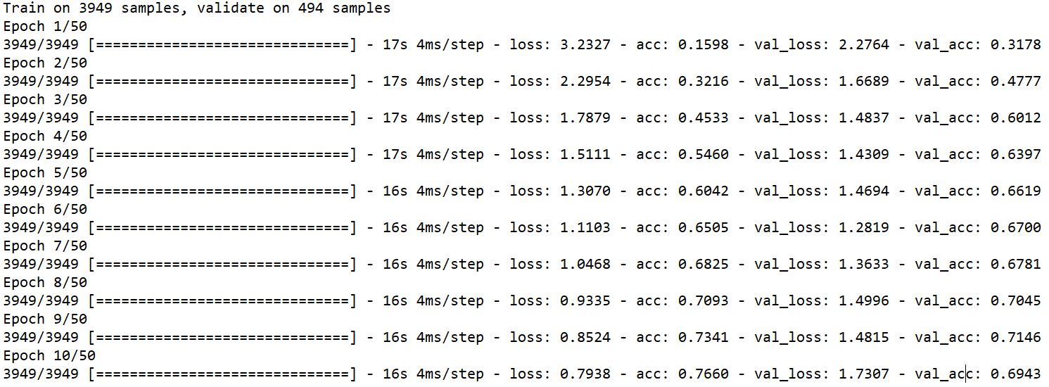
There is a mismatch between the lowest loss achieved in epoch 6 and the highest accuracy on the validation set achieved in epoch 9. This can be explained by the way classification works if the model is managing to classify a larger number of the validation set, but with lower confidences as the model begins to over fit, we would expect this pattern to occur. We would like our identifications to be robust when we move to the test set, so we shall select the epoch with the lowest loss. Accordingly we train our model again, this time just for 6 epochs and get the following output.
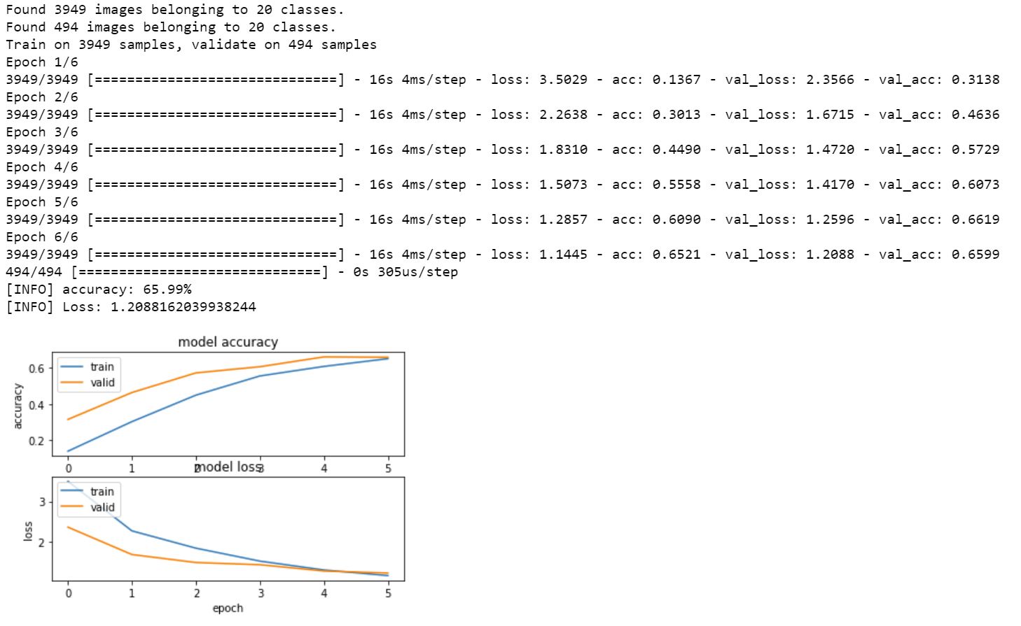
This looks fairly reasonable for a first attempt at classifying 20 categories of very similar looking LEGO images. Our accuracy is 66% which is well in excess of chance for the categories (20 categories = 5%). We could go back and increase our sample set via data augmentation or tweak the layers in our model but for the purposes of this tutorial this outcome is sufficient. Our next step is to use the model to classify our test set.
The excellent pre-existing tutorial on using transfer learning with the VGG16 model only lets us categorise one image at a time. Lets write some different code so that we can apply the classifier to a collection of images one after another. Lets start by creating a function to load the model so that we can use it
def build_model2(class_dictionary, num_classes):

    # build the VGG16 network
    model1 = applications.VGG16(include_top=False, weights='imagenet')
    #model2 = applications.VGG16(include_top=False, weights='imagenet')

    # build top model
    model2 = Sequential()
    model2.add(Flatten(input_shape=(7, 7, 512))) # (7, 7, 512) bottleneck_prediction.shape[1:]
    model2.add(Dense(256, activation='relu'))
    model2.add(Dropout(0.5))
    model2.add(Dense(num_classes, activation='sigmoid'))

    model2.load_weights(top_model_weights_path)
    return model1, model2
Next lets write a function to conduct a prediction for a single image
</pre>
def prediction2(image_name, class_dictionary, model_1, model_2):

    # add the path to your test image below
    image_path = image_name

    orig = cv2.imread(image_path)

    print("[INFO] loading and preprocessing image...")
    image = load_img(image_path, target_size=(224, 224))
    image = img_to_array(image)

    # important! otherwise the predictions will be '0'
    image = image / 255

    image = np.expand_dims(image, axis=0)

    # get the bottleneck prediction from the pre-trained VGG16 model
    bottleneck_prediction = model_1.predict(image)

    # use the bottleneck prediction on the top model to get the final
    # classification
    class_predicted = model_2.predict_classes(bottleneck_prediction)

    probabilities = model_2.predict_proba(bottleneck_prediction)

    inID = class_predicted[0]

    inv_map = {v: k for k, v in class_dictionary.items()}

    label = inv_map[inID]

    # get the prediction label
    return label
With this done lets create a list of the locations of our test images on disc
test_image_paths = []
test_image_directories = []

test_image_directories = os.listdir('data/test/')

for directory in test_image_directories:
    test_images = os.listdir('data/test/'+ directory)
    for timage in test_images:
        test_image_paths += [('data/test/'+ directory + '/' + timage, directory)]

print (len(test_image_paths))
print (test_image_paths[3])
This creates a list of tuples of test image locations and the correct label for each image. Now we are almost ready to start doing some predicting. Lets load the class indices, calculate the number of classes, and then iterate over the pictures we want to classify and get our model to predict which category the LEGO picture belongs to
</pre>
true = 0
total = 0

# load and calculate our constant variables
class_dictionary = np.load('class_indices.npy').item()
num_classes = len(class_dictionary)
model_1, model_2 = build_model2(class_dictionary, num_classes)

for candidate in test_image_paths[0:450:10]:
    answer = prediction2(candidate[0], class_dictionary, model_1, model_2)
    print ("Actual: "+ candidate[1] + " Predicted: " + answer)
    total += 1
    if candidate[1] == answer:
        print ("true")
        true +=1

print ('Percentage correct = ' + str(true/total*100))
<pre>
As this is a test set with labels, we can also get the classifier to compare its prediction to the ground truth for each image so that it can tell us the percentage accuracy of classification. When we run it on all our test images we get 65.7%, accuracy. This very close to our validation set, giving us good confidence that our model is robust. As usual the code can be found on Github.
Why does accuracy peak at around 66% for this model. Well firstly the classes are very similar, our VGG16 bottleneck network is good at extracting features, but not necessarily the correct ones to differentiate between different kinds of LEGO. Secondly looking at some of the failure cases it can be seen that they do indeed look pretty similar to other categories, who knew LEGO could be so tricky?
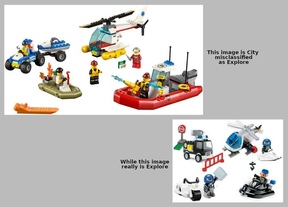
We could try to improve the accuracy by training a full model or by data augmentation, but some of the edge cases would likely remain hard to classify. This model has demonstrated that it can do a reasonable job of classifying LEGO images from BrickSet. And as for that tractor back in part 1.
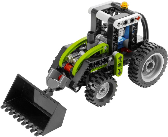
Lets place a copy of the image on its own in the /data/test/Technic/ folder and run our algorithm on it
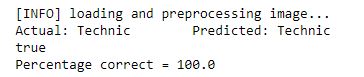
Totally Technic LEGO!