A lot of datasets include rows with missing values. These values rows either need to be removed or the missing values need to be approximated. MICE (Multiple Imputation by Chained Equations) is a neat way to infer more accurate values for missing data in a dataset. The basic idea is to use simple machine learning models to calculate missing values. The way this is done is to first fill missing values with column averages and then use machine learning models to calculate better approximations for the missing values. Generally the model derived estimates for the missing values are then fed back to the model in a loop for a number of iterations to provide better and better estimations of the missing values.

A simple way to do this in pandas is to use the miceforest library. Despite its name miceforest actually uses LightGBM based trees rather than random forests to calculate the missing values. This should allow it to better handle large datasets, sparse features and data with high dimensionality.
Types of Missing Data
An important consideration when imputing values is to consider the distribution of the missing values. There are three main possibilities for the missing values:
- MCAR – Missing Completely at Random: The values which are missing are in no way dependent on what their value would have been had they not been missing. For example, missing data randomly dropped from a data stream
- MAR – Missing at Random: The missing data is dependent on other observed variables but not the missing variable itself. For example, if women are less likely to report their marital status in a survey than men
- MNAR Missing Not at Random: The missing data is dependent on the value being predicted. For example if older people are less likely to report their age
A common warning is that it can be dangerous to use MICE for imputation on MNAR data. In these cases more advanced approaches such as Heckman corrections should be used instead. You can of course roll your own Heckman models in Python. However using an available library is often more convenient for initial experiments on a new dataset. Therefore I decided to perform a few experiments with synthesised missing data for each of the three kinds of missing data. The aim was to see what sort of performance could be expected at a variety of levels of missing data with miceforest.
The Experiment
To get a feel for this, I set up a simple Google Colab workbook which introduces the three different types of errors into the feature columns of the classic Iris dataset. Once this is done the workbook imputes the missing data and then compares the performance of miceforest to simple averages. The workbook examines each column in isolation. However because I normalised the column values, we can get an indicative feeling for relative performance by looking at the averaged MAE and RMSE across the columns for different levels of missing values.
As you can see in these plots, MICE generally outperforms averaging by a significant margin. The performance advantage does fall off as the volume of missing values becomes high. At most likely levels of missing values however MICE appears to have a clear advantage in practice even for MNAR data. These images are Mean Absolute Error but the workbook also includes RMSE plots.
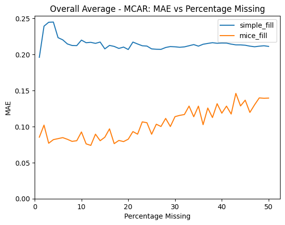
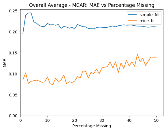
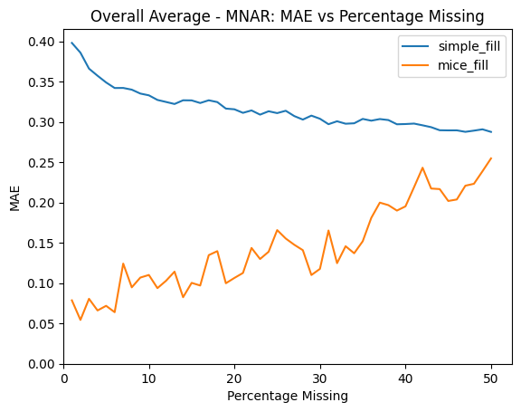
This can be seen even more clearly if we look at graphs of the percentage advantage MICE has compared to averages. In these graphs the advantage in terms of both RMSE and MAE is depicted.
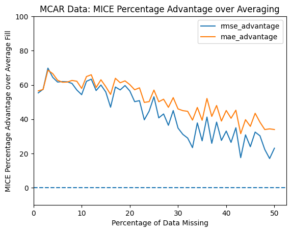
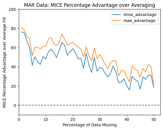
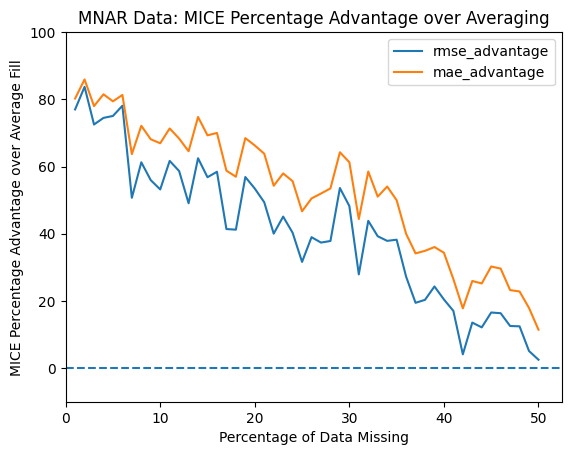
Note that for all these graphs approximately half of the influence on missingness is random and half due to the value of the influencing column in the case of MAR and MNAR data. There is a tuneable value in the workbook to allow for different levels of influence so you can always take a copy of the workbook if you wish to investigate that aspect, but I found that the same general rule of thumb held true for a wide variety of values. Likewise you can decide how many rounds of MICE to use (the graphs used 10) but even low values like two rounds show considerable improvement over average imputation.
Its worth noting that some individual columns in the source data do not display such a clean improvement, but as a general strategy MICE seems to outperform averaging at low missing rates.
Conclusion
I think that these results show that while there may be better ways to impute data if you suspect it is MNAR, miceforest will give pretty decent results. For most realistic data sets for initial data modelling exploration it is likely a useful starting point. you can then decide whether your data requires more bespoke null imputation.
